Contents
clc;clear;close all;
Set the system constants as global variables that may be used by other functions
global Crr M g CdA rho Iw rw MPH2mps Mgvwr
System Constants
All system constants are defined here. These pertain to the glider.
Crr = 0.009;        %[], coefficient of rolling resistance of the tires
M = 1500;           %[kg], mass of the vehicle
g = 9.81;           %[m/s/s], gravitational constant
Cd = 0.35;          %[], coefficient of aerodynamic drag for the vehicle
A = 2;              %[m^2], frontal area of the vehicle
CdA = .75;          % product of the drag coeff. and frontal area
rho = 1.2;          %[kg/m^3], density of air at STP
Iw = 0;             %[?], moment of inertia of a wheel/tire on the vehicle
rw = .32;           %[m], effective rolling radius of the tire
MPH2mps = .44704;   % The EPA profiles are provided with MPH as the unit for the speed. This is used to convert back to m/s.
Mgvwr = 2000;
Load the drive cycles of interest
This function loads any drive cycle of interest and then converts the speed to m/s.
fileNames = {'hwycol.txt','us06col.txt','uddscol.txt'};
fns = {'hwy','us06','udds'};
[v_prof.hwy, v_prof.us06, v_prof.udds] = loadProfiles(fileNames);
EcoCAR3 - Problem 1 - Wheel energy and performance analysis
[Out] = vehEnergy(v_prof,'wheel');
[Out] = vehPerf('wheel');
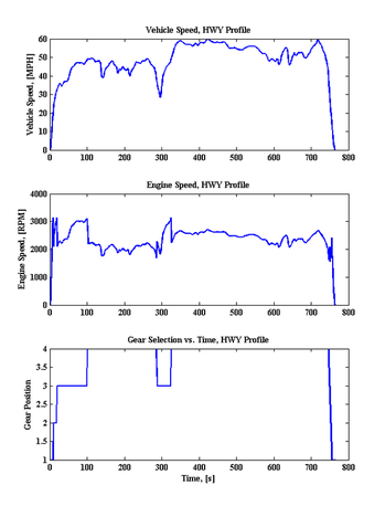
EcoCAR3 - Problem 2 - Conventional vehicle energy and performance analysis
[Out] = vehEnergy(v_prof,'conv'); mk_comp_fig_pos = [16,59,650,736]; gtl_sim_comp = [102,120,650,943]; % Loop through plotting the data for the drive cycles. for i = 1:length(fns) fn = fns{i}; % Set the file name based on the loop increment. fig1=figure(i); % Create a figure window and set a name for that window for later manipulation. set(fig1,'outerposition',mk_comp_fig_pos); % Set the figure window outer screen position lw=2; % Set the linewidth to be used for plotting. subplot(3,1,1);plot(Out.conv.veh_spd.(fn)(:,1),Out.conv.veh_spd.(fn)(:,2)/MPH2mps,'linewidth',lw); % Subplot 1 of the vehicle speed.. ylabel('Vehicle Speed, [MPH]');title(['Vehicle Speed, ' fn ' profile']); % Set the x and y axis labels along with the title. subplot(3,1,2);plot(Out.conv.veh_spd.(fn)(:,1),Out.conv.eng_spd.(fn),'linewidth',lw); ylabel('Engine Speed, [RPM]');title(['Engine Speed, ' fn ' profile']); subplot(3,1,3);plot(Out.conv.veh_spd.(fn)(:,1),Out.conv.gear.(fn),'linewidth',lw); xlabel('Time, [s]');ylabel('Gear Position');title(['Gear Selection vs. Time, ' fn ' profile']); fig=gcf; set(findall(fig,'-property','FontWeight'),'FontWeight','Bold') % Set the figure font weight to bold end % Average full load engine efficiency is ~35% for the engine selected. % Hence using the wheel load analysis, the conventional vehicle will % require wheel_power_avg/eta_avg % Out.conv.avg_power_zts = Out.wheel.avg_power_zts/avg_eng_eta; % Out.conv.avg_power_grade = Out.wheel.avg_power_grade/avg_eng_eta; % %% EcoCAR3 - Problem 3 - Electric vehicle energy and performance analysis % [evNrg_hwy,evNrg_us06,evNrg_udds] = vehEnergy([v_prof_HWY, v_prof_US06, v_prof_UDDS],'ev'); % [ev_perf] = vehPerf('ev'); % %% EcoCAR3 - Problem 4 - Series hybrid electric vehicle energy and performance analysis % [shevNrg_hwy,shevNrg_us06,shevNrg_udds] = vehEnergy([v_prof_HWY, v_prof_US06, v_prof_UDDS],'shev'); % [shev_perf] = vehPerf('shev');
