Master file for simulating the quarter car model.
Name: Matthew Klein, Contact: [email protected], Date: 3/28/14
Contents
Clear old data, Designate global variables
clear; close all; clc;
global A B v_in dt g
System Parameters
System Constants
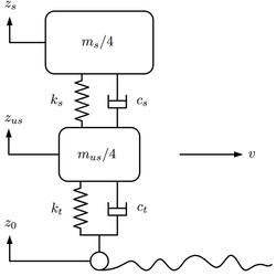
g    = 9.81;                                % [m/s^2]
 % masses
m_s  = 1500/4;                              % corner mass is 1/4th the full mass, [kg]
m_us = m_s/7;                               % 1/7th the body corner mass, [kg]
 % springs - The displacements are intuitively derived in order to create
 % relatively realistic stiffness values for the compliance elements.
d_s  = 2*.0254;                             % equilibrium displacement of spring, [m]
d_t  = d_s/5;                               % equilibrium displacement of tire, [m]
k_s  = m_s*g/d_s;                           % Spring stiffness, [N/m]
k_t  = (m_s+m_us)*g/d_t;                    % Tire stiffness, [N/m]
 % damping - a damping ratio of 0.5 was selected.  This is a common value
 % for automotive suspensions as it balances cornering traction with comfort.
zeta = 0.5;                                 % Damping ratio
b_c  = 2*sqrt(k_s*m_s);                     % Critical damping coefficient
b_s  = zeta*b_c;                            % Damping coefficient
b_t  = .1*2*sqrt(k_t*(m_s+m_us));           % ~false tire damping for numerical stability
System Matrices
State transition matrix
A = [-b_s/m_s,  b_s/m_us,       k_s, 0;     % p_s
      b_s/m_s,(-b_s-b_t)/m_us, -k_s, k_t;   % p_us
     -1/m_s,    1/m_us,         0,     0;   % q_s
      0,       -1/m_us,         0,     0];  % q_t
% Input matrix
B = [0, -m_s; b_t, -m_us; 0, 0; 1, 0];      % u = [v_in(t); g]
Time vector
Setup the time step and end time
dt_ratio = 20;                  % ratio of time steps to fastest eigenvalue of the system matrix
tau_fast = abs(1/max(eig(A)));  % fastest system time constant, [seconds]
dt       = tau_fast/dt_ratio;   % time step size, [seconds]
t_end    = 5;                   % end time, [seconds]
time     = (0:dt:t_end)';       % simulation time vector, [seconds]
Creat the input vector
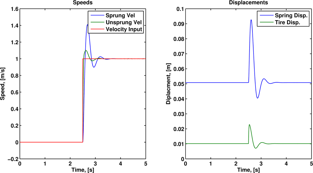
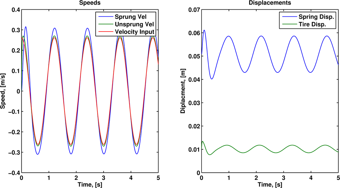
The velocity input time profile is generated. Two different profiles may be used. Set test_type to 0 for a step input, or to 1 for a sinusoidal input. The sinusoidal velocity input is derived from an arbitrary road profile.
U    = 25;                      % forward velocity, [m/s]
a_d  = .05;                     % amplitude of road displacement, [m]
d_b  = 30;                      % bump spacing, [m]
test_type = 0;
if test_type == 1
    % x_in = a*sin(b_d*x) then take the time derivative ->
    v_in = (2*pi/d_b)*U*a_d*cos((2*pi/d_b)*U*time); % velocity input, [m/s]
    test = 'sinusoidalInput';
else
    % Use for step velocity input
    v_in = zeros(length(time),1);
    v_in(round(length(v_in)/2):end) = 1;
    test = 'stepInput';
end
Initial conditions
There are four states for this system. The two momenta, which will be initialized as 0 (no initial speed for the masses) and the equilibrium displacements for the two compliance elements.
x_0 = [0, 0, 1/k_s*m_s*g, 1/k_t*(m_s + m_us)*g];
Call the ODE solver
We are using ode45, which is the solver that you will most likely use. It is a great first solver to try. There are many solvers in MATLAB and you can search for 'ode solvers' in the product help to learn more about those.
[t_out, x_out] = ode45(@Lab1_eqns, time, x_0);
Create outputs
Create the C matrix and then compute the output vector using the full state information from the ODE solver.
C = [1/m_s, 0,      0, 0;   % output 1: v_s
     0,     1/m_us, 0, 0;   % output 2: v_us
     0,     0,      1, 0;   % output 3: displacement of spring
     0,     0,      0, 1];  % output 4: displacement of tire
y = zeros(size(x_out));
for i = 1:length(time)
    y(i,:) = x_out(i,:)*C';
end
Plot the data
The plot commands below are the ones I use for generating publication quality figures, which you will all need to learn how to do. Particularly for the PhD students here.
plots_on = 0; % I use this as a quick way to stop plotting.  It's particularly nice for me during debugging.
if plots_on
    F1 = figure(1);                                             % Create a figure window and assign it to a handle, F1 here.
    lw = 1; FN = 'Arial'; FS = 12; FW = 'bold';                 % Create variables for the linewidth, font name, font size and font weight
    set(F1,'units','inches','OuterPosition',[4.5 1 11.5 6.5]);  % Set the figure window size using the figure handle F1

    sp1=subplot(1,2,1);                                         % Create a subplot
    plot(time,[y(:,1:2),v_in],'linewidth',lw);                  % add a plot to the subplot and specify the linewidths
    legend('Sprung Vel','Unsprung Vel','Velocity Input');       % Create a legend
    xlabel('Time, [s]','Fontsize',FS,'Fontname',FN,'Fontweight',FW);        % Create an x-axis label
    ylabel('Speed, [m/s]','Fontsize',FS,'Fontname',FN,'Fontweight',FW);     % Create a y-axis labe
    title('Speeds','Fontsize',FS,'Fontname',FN,'Fontweight',FW);            % Create a title for the sublot
    set(gca,'Fontsize',FS,'Fontname',FN,'Fontweight',FW,'linewidth',lw);    % Set the current axes fonts and linewidths

    sp2=subplot(1,2,2);                                         % Create a second subplot
    plot(time,y(:,3:4),'linewidth',lw);
    legend('Spring Disp.','Tire Disp.');
    xlabel('Time, [s]','Fontsize',FS,'Fontname',FN,'Fontweight',FW);
    ylabel('Diplacment, [m]','Fontsize',FS,'Fontname',FN,'Fontweight',FW);
    title('Displacements','Fontsize',FS,'Fontname',FN,'Fontweight',FW);
    set(gca,'Fontsize',FS,'Fontname',FN,'Fontweight',FW,'linewidth',lw);

    nameFig1=['Lab1Demo_' test '_032714'];                                  % Create a name for the figure file
    export_fig([nameFig1,'.png'],'-transparent','-r300','-painters');       % Save a 300dpi version of the figure in png format using the expot_fig function.
end
